This past weekend I set aside some time to do a deep dive into neural networks, specifically the smallest components, building a ground up neural network from scratch in Julia. This article will roughly cover the first episode of Andrej Karpathy’s “Zero to Hero” series. Also, you can find his implementation of micrograd on github. I’ll be building writing our own;with a compute graph, basic neural network, and training functionality.

You can follow along by downloading my Pluto.jl notebook here

Before we jump into building a neural network, we first need two things: a representation of a computational graph, and a method to perform backpropagation.

Starting with the computational graph, the smallest unit of our micro neural network is the Value. This structure keeps track of a few things, the current value, the gradient, a callback function for backwards propagation, and children. The operation field is included for display purposes. For now, the only important field here is the scalar.

Base.@kwdef mutable struct Value
    scalar::Real = 0.0
    grad::Real = 0.0
    back::Function = (() -> Nothing)
    children::Tuple = ()
    operation::Union{Nothing,Symbol} = nothing
end
Value(s::Real; kwargs...) = Value(scalar=s; kwargs...)
Value(s::Real, g::Real; kwargs...) = Value(scalar=s, grad=g; kwargs...)

We’re using the Base.@kwdef macro here to code gen a structure with default values and writing some helper functions to make construction easier. We next define some basic numeric operations. Addition +, Subtraction -, Multiplication *, and Exponentiation ^.

Numerically, these functions simply compute the numeric operation between two values. Via the children field, these functions will also build a computational graph, later allowing us to trace backwards (via backpropagation) and to calculate an individual value’s gradient.

function Base.:+(a::Value, b::Value)
    out = Value(a.scalar + b.scalar, children=(a,b), operation=:+)
    out.back = function()
        a.grad += out.grad
        b.grad += out.grad
    end
    return out
end

function Base.:-(a::Value, b::Value)
    out = Value(a.scalar - b.scalar, children=(a,b), operation=:-)
    out.back = function()
        a.grad += out.grad
        b.grad += out.grad
    end
    return out
end

function Base.:*(a::Value, b::Value)
    out = Value(a.scalar * b.scalar, children=(a,b), operation=:*)
    out.back = function()
        a.grad += (b.scalar) * out.grad
        b.grad += (a.scalar) * out.grad
    end
    return out
end

function Base.:^(a::Value, b::Real)
    out = Value(a.scalar^b, children=(a,), operation=:^)
    out.back = function()
        a.grad += b * (a.scalar ^ (b - 1)) * out.grad
    end
    return out
end

Ignoring the out.back lines for now, these functions will propagate the computation of values a and b through the different operations. For example we can now combine operations to make complex computational graphs.

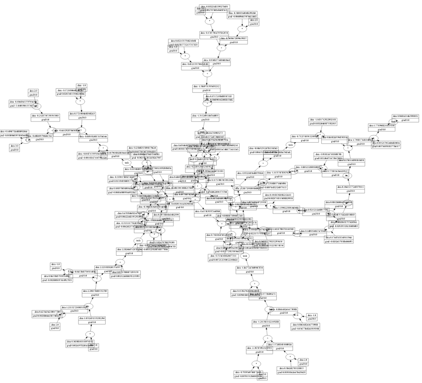
a = Value(2)
b = Value(3)
a + b
>>> Value(scalar=5, grad=0.0)

With a helper function (see full notebook), we can display the computation graph via graphviz:

In order for these values to play nicely with other Number types, we’ll need to define some functions that wrap regular numbers with out Value type.

Base.:+(a::Value, b::Real) = a + Value(b)
Base.:+(a::Real, b::Value) = Value(a) + b
...
and so on

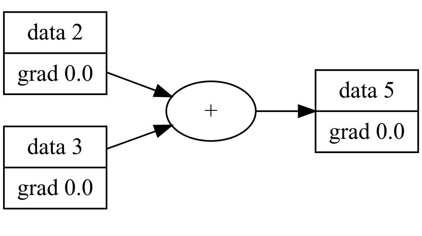
a = Value(2)
b = Value(3)

d = (a + b)*4
>>> Value(scalar=20, grad=0.0)

Notice how the 4 is converted neatly into it’s own Value? Nice right?

Backward Propagation

If you take what we’ve implemented and compute the final value of our graph, you’ll be doing forward propagation. That is: calculating the output with respect to the inputs. Backward propagation is all about computing the “contribution” that an input has to a system or equation with respect to the output.

We know from high school calculus that continuous functions have what’s called a “derivative”. We have various rules for computing the derivative of a function symbolically, like 2x^2+3x+4 is 4x+3. The derivative, also written dx/dy or “how much a change in x affects the change in y” will be critical to determining how specific parameters (or inputs) contribute to the overall “wrongness” of our model’s output.

Backpropagation (or backprop) uses the chain rule to combine multiple function’s derivatives together. Meaning, if we can define a single operation’s local derivative, we can define more complex operations and differentiate them automatically. This is called Differentiable Programming and specifically we’re taking the “Operator overloading, dynamic graph” approach.

Programmatically, this is done by iterating through the graph in a reverse topographical manner, computing each parameter’s gradient (derivative) step-by-step using the previous value’s gradients. It’s important to note that backwards propagation will only modify the gradient component of our Values where as forward propagation only computes the scalar component. Our training step will use both of these values to train our model.

function backprop(v::Value)
    topo = []
    visited = Set()
    function build_topo(root)
        if root ∉ visited
            push!(visited, root)
            for child in root.children
                build_topo(child)
            end
            push!(topo, root)
        end
    end
    build_topo(v)
    
    v.grad = 1.0
    for node in reverse(topo)
        node.back()
    end
end

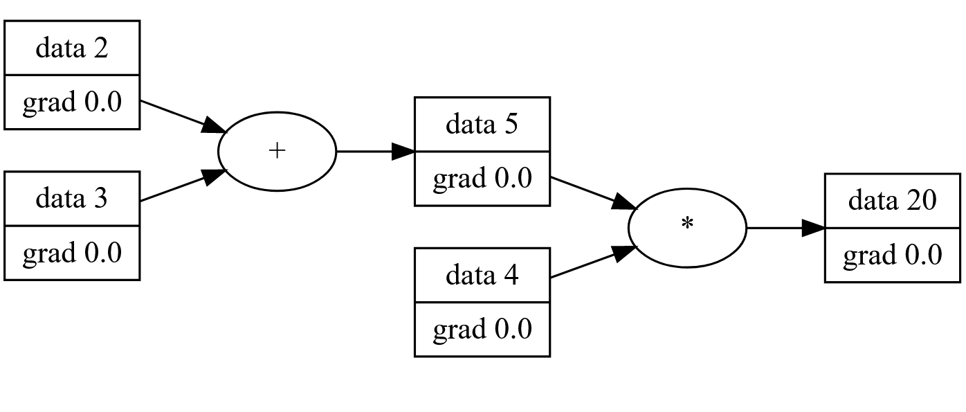
I won’t go over the topographic sort section, but I’d like to point out how simple the backprop function is because we’ve done all the work in defining each derivative at the operator level. The only thing that this function is really doing is ensuring we compute the gradients in the correct order.

For our simple network (a + b)*4 we can see the gradients after backprop:

Building a Neural Network

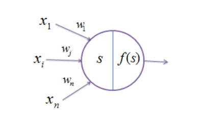
Next, we’ll be designing a Multi-layer Perceptron, a type of classifier that’s simple and surprisingly capable when it comes to solving problems. A Neuron is a rough analog to it’s biological counterpart, which takes in a list of values and outputs a single value based on some activation function. For now, the architecture and activation functions aren’t necessarily important, what’s important is how we implement them using our Value system which will allow us to perform backprop (differentiation) automatically.

A multi layer perceptron is composed of many layers, which are composed of neurons, we’ll define this structure below. We’re initializing all our Neuron’s weights randomly, and setting the bias to zero.

mutable struct Neuron
    weights::Vector{Value}
    bias::Value
end

function Neuron(nin::Int)
    weights = [Value(scalar=rand(Uniform(-1,1))) for _ in 1:nin]
    bias = Value(scalar=0)
    Neuron(weights, bias)
end

mutable struct Layer
    neurons::Vector{Neuron}
end

Layer(nin::Int, nout::Int) = Layer([Neuron(nin) for _ in 1:nout])

mutable struct MLP
    layers::Vector{Layer}
end

function MLP(nin::Int, nouts::Vector{Int})
    sz = vcat(nin, nouts)
    layers = [Layer(sz[i], sz[i+1]) for i in 1:length(nouts)]
    MLP(layers)
end

Each Neuron is composed of N weights and a bias. These are combined linearly wx+b and passed through an non-linear activation function, in our case tanh which signals every neuron in the next layer. Since this is just another operation, we will need to implement the derivative, which I’ve stolen from Wikipedia.

# activation function
function tanh(v::Value)
    x = v.scalar
    t = (exp(2x) - 1) / (exp(2x) + 1)
    out = Value(scalar=t, children=(v, ), operation=:tanh)
    out.back = function()
        v.grad += (1 - t^2) * out.grad
    end
    return out
end

# forward propagation
function (n::Neuron)(x::Vector)
    # wx + b
    act = sum(n.weights .* x) + n.bias
    out = tanh(act)
    return out
end

function (l::Layer)(x::Vector) 
    outs = [n(x) for n in l.neurons]
    return length(outs) == 1 ? outs[1] : outs
end

function (mlp::MLP)(x::Vector)
    for layer in mlp.layers
        x = layer(x)
    end
    return x
end

Note: the line n.weights .* x is doing a vector operation, applying the multiplication operator to each pair of values in the weight and input. Similar to map((a,b) -> a*b, zip(n.weights, x))

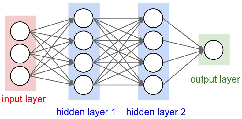
The forward pass involves computing each layer sequentially, passing the output of each layer to every other layer in the next step. Each layer is computed by passing all of the previous layer’s signals into each neuron. For example a MLP(3, [4,4,1]) model has a 3-neuron input layer, two 4-neuron “hidden” layers and a single neuron output. This is a type of fully-connected neural network.

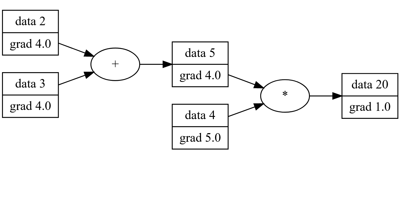
Here’s our entire neural network, represented in Values after running a forward pass:

Training and loss

Now that we have a basic neural network implemented, it’s time to train it.

xs = [
    [2, 3, -1],
    [3, -1, 0.5],
    [0.5, 1, 1],
    [1, 1, -1],
]
ys = [1, -1, -1, 1]

model = MLP(3, [4,4,1])

Let’s take a simple example. We build a Multi-layer Perceptron that accepts 3 dimensional input, and passes that through a series of hidden layers that ultimately results in a single layer which provides us a single scalar. This is also known as a classifier.

We provide 4 example inputs, and their corresponding outputs. The xs dataset contains those three dimensional inputs we mentioned earlier, and ys is the list of singular scalar outputs.

We can use this fresh model to predict (although not particularly well) what it thinks the outputs should be given the inputs.

>>> scalar.(model.(xs))

4-element Vector{Float64}:
 0.8701960396200752
 0.8645974266020415
 0.8645974266020415
 0.7925291442209874

So far, not so great considering our “correct” values are [1, -1, -1, 1]

We need a method to quantify how good or bad our model’s guesses are. This is called a Loss Function and we’ll stick to a rather simple one, the Mean Squared Error. It’s important to note that this loss function is NOT a simple value, rather, it’s the entire network of computations that the model had to make in order to make a decision. This is what allows our backprop step to work.

This loss function will take the squared difference between the correct value and the predicted one. When we talked about back propagation, we want to know how each parameter in the computational graph contributes to the total outcome. The key insight here, is by using our graph of Values we can directly calculate this contribution via backwards propagation. In other words, we now have a gradient that tells us directly how much a specific parameter contributes to the overall “wrongness” of the model’s predictions.

If you noticed earlier, forward propagation and backward propagation are operating on separate values scalar and grad. This last step, known as Gradient Descent ties the two together. We take our gradient values from the loss function, and use those gradients to “nudge” each parameter in the right direction by a fixed rate, also called the learning rate.

for k in 1:10
    # forward propagation
    # make a prediction
    scores = model.(xs)

    # compute the loss
    # determine how "wrong" our model is
    sum((scorei - yi)^2 for (yi, scorei) in zip(ys, scores))
    
    # zero grad will remove previous run's gradients, as they're computed
    # cumulatively per backprop.
    zero_grad(model)

    # Use our backprop algorithm to determine
    # how much each parameter contributes to the "loss" (gradients)
    backprop(loss)

    # Use these gradients to "nudge" our weights and biases around
    # hopefully minimizing the loss function overall.
    learning_rate = 0.05
    for p in parameters(model)
        p.scalar += learning_rate * p.grad
    end
    println("step $k, loss $(loss.scalar)")
end

This “nudge” will eventually move each parameter towards a local minimum which will minimize the overall loss, meaning our model should become less and less wrong each time we iterate.

When performed iteratively:

• Run Forward Propagation
• Calculate the loss function
• Run Backward Propagation on this loss, calculating each parameter’s gradient
• Use this gradient to nudge all parameters in the right direction.

step 1, loss 1.8513252792660841
step 2, loss 1.1349644835442254
...
step 48, loss 0.03086321842845595
step 49, loss 0.030156185155040656
step 50, loss 0.02947950948849564

After 50 (arbitrary) steps. We see that the loss has been minimized to 0.0294 , we can now check the predictions to see how close they are to the desired:

scalar.(model.(xs))
4-element Vector{Float64}:
  0.9218994725231098
 -0.8884333726789942
 -0.9511039076622398 
  0.9111536386687518
ys
4-element Vector{Int64}:
  1
 -1
 -1
  1

Very nice! This is much closer to our expected outputs. Our model has effectively learned the hidden function y=f(x)!

I’ve shown that through a bottom up approach using some basic calculus that you can write your own neural network from scratch. This is only the tip of the iceberg, however, our simple model works for simple datasets, but will need a lot better model architectures and tuning than we have time for today.

For example there’s an entire field of research into writing precise and performant loss functions, how to control learning rates, when to batch data for faster learning, etc. My hope is that this has at least inspired you to dive a bit deeper into neural networks.

Thanks for reading.